
Gliders and Riders A Particle Swarm Selects for Coherent Space-time Structures in Evolving Cellular Automata by Jeffrey Ventrella (created in 2005 - this page updated in 2009)
Download the chapter published in
Stigmergic Optimization

Download the paper published in Alife X, 2006 
|
|
|
Let's Evolve Gliders
Cellular automata (CA) play an important role in the history of artifial life research. The most popular CA is the Game of Life. Gliders are coherent space-time structures that arise within the primordial soup of CA. Most CA rules do not produce gliders, but those that do have been studied quite a bit (class 4 CA). Gliders can be considered as vehicles which move information, and they are present in CA which support universal computation. The notion that simple rules, when applied repeatedly over time, can give rise to universal computation is quite compelling, and so is the question of how to evolve rules that generate gliders. In searching for a technique to test CA dynamics for gliderhood, I explored using traditional pattern-recognition techniques. I wanted to create the algorithmic equivalent of smooth eye-tracking - and the natural ability for the eye-brain system to detect coherent motion in an otherwise noisy background. I settled on the idea of using particles with inertia. Consider your visual focus on a noisy chaotic field of motion as a 'particle'. That particle can be pulled along when it detects some coherent motion. That is the basic motivation for developing this technique. |
|
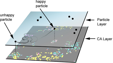
Marbles on a Tile Floor
Let's shift to another metaphor now. Imagine a large kitchen floor with square tiles. Each tile is a different color. Now imagine rolling a marble across the floor. Imagine that the kitchen floor is actually a cellular automaton - the colors of the tiles are constantly changing according to CA rules - in fact, they are changing colors about 30 times a second. The marble is magnetically attracted to certain colors, and it gets pulled around the floor as the tiles change colors. Now, imagine that the marble is 'happy' when it is moving in a straight line. When the marble is happy, it says, "I like what these tiles are doing to me." |
Hold on to this little narrative about the marble on the magic kitchen floor. It will help as I explain how this scheme works. Now let's get a whole bag of marbles. This bag of marbles will serve as a kind of particle swarm. At the start of the simulation, each cell (tile) has its own rule - determined randomly. And the states (tile colors) are also set randomly. This means that at the start, the colors will start changing chaotically. The bag of marbles is tossed onto the kitchen floor, and they begin to roll around aimlessly. So far, these are very unhappy marbles! |
|
|
|
But Wait...These Marbles Have a Plan
The swarm of particles (bag of marbles) has the ability to alter the rules of the cells (tiles) that they are rolling over. In addition to that, each particle has the ability to record the rule of the cell it is rolling over. Particles record rules when they are happy (when they are having a nice ride), and they distribute those rules onto other cells around as they roll over them. This means that the particle swarm has the ability to change the rules over time such that they end up moving in straight lines more over time. Without ever explicitly designing the CA rules up front to generate gliders, the particle swarm encourages gliders to emerge spontaneously, by way of their ability to alter the rules over time. |
CA, PSO, and GA
This simulation is called "Gliders and Riders", because it evolves gliders and this happens because the particle swarm "rides" along the backs of gliders. It combines three algorithmic domains commonly used in artificial life: (1) Cellular Automata (CA), (2) Particle Swarm Optimization (PSO), and (3) the Genetic Algorithm (GA). The genetic algorithm is basically the scheme by which the rules associated with each tile (cell) changes. And the genetic operators are performed by the particle swarm. Instead of using a standard genetic algorithm on a population of rules (applied uniformly on all cells of a CA), the particle swarm interacts intimately with each cell in its local region, and performs genetic operators as the dynamics emerge. |
|
|
|
Stigmergy
The swarm selects for local dynamics that support coherent motion. Unlike standard particle swarms, these particles do not fly on a search mission � instead, they ride on the backs of clusters of emerging structures, due to attractive forces. |
In exchange for a good ride, they reward local dynamics with more coherent motion by performing genetic operators of selection and reproduction. This technique not only demonstrates an efficient way to evolve a huge variety of gliders, it also acts as a simulation of emergent complexity, and employs the principle of stigmergy. |
|
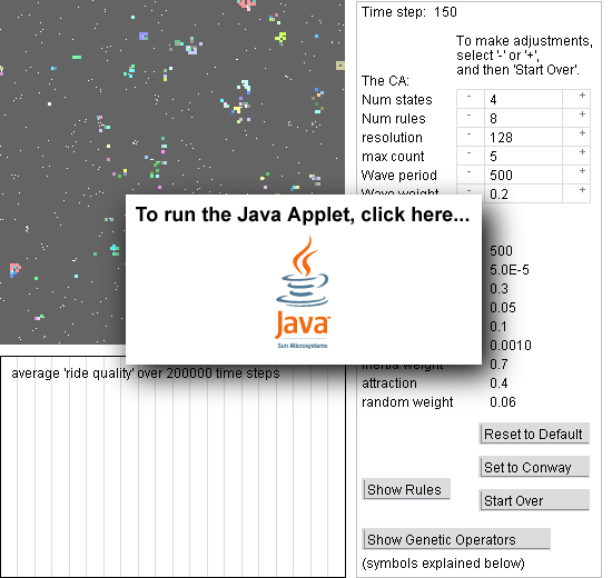
About the Java Simulation The simulation will run for 200,000 time-steps. The speed of the simulation depends on the computer. Running on a faster computer is recommended, if possible. Most of the resulting dynamics will be of the "Brain" variety, having various forms of gliders and linear waves propagating at the speed of light in all four orthogonal directions. Other varieties of glider-rich CA dynamics can evolve as well. The white dots are the particles. The cells in the CA are colored differently for each state, as determined by genes. The quiescent state is shown as gray. Although these color values are genetic, they do not have any evolutionary purpose - they are there to serve human eyes only. The Graph The graph just underneath the simulation shows the progress of the swarm over the span of the 200,000 time steps. What it shows is the value of "average ride quality" of the particles WHICH ARE RIDING. In other words, if a particle is being attracted to a cluster of live cells, it is said to be "riding" on that cluster. If that cluster of live cells is moving at a coherent velocity, the particle measures this as a "good ride", and then rewards the local region of the CA with selection and reproduction. When the graph is updated (every 500 time steps) the "ride quality" of each particle that is riding is measured and averaged into one single value. This value is what is plotted in the graph. Average ride quality increases as gliders emerge. Symbols Visualizing the Genetic Operators A toggle button is provided for turning on or off the view of the genetic operators that the particles perform. These are as follows:  Selection - a particle selects a copy of the genes of its reference cell when it has detected a superior ride. This is
shown as a dot appearing at the location of the particle.
Selection - a particle selects a copy of the genes of its reference cell when it has detected a superior ride. This is
shown as a dot appearing at the location of the particle.
 Reproduction - All particles continually deposit copies of the genes they carry around back into the CA space. When
depositing genes, crossover is used, such that contiguous sections of the gene sequence is copied onto a Moore
neighborhood surrounding the reference cell. This is shown as a horizontal line appearing at the location of the particle.
Reproduction - All particles continually deposit copies of the genes they carry around back into the CA space. When
depositing genes, crossover is used, such that contiguous sections of the gene sequence is copied onto a Moore
neighborhood surrounding the reference cell. This is shown as a horizontal line appearing at the location of the particle.
 Exchange - When two cells come in contact with each other (reach within a cell's-width of distance), there is a random
chance of exchanging genetic information. The particle which has detected a superior ride gives a copy of its genes to
the other particle. This is shown as a vertical line appearing at the location of the particle.
Exchange - When two cells come in contact with each other (reach within a cell's-width of distance), there is a random
chance of exchanging genetic information. The particle which has detected a superior ride gives a copy of its genes to
the other particle. This is shown as a vertical line appearing at the location of the particle.
 Mutation - Every cell has a (rare) chance of having one of its genes randomly changed. This is shown as an 'x' which
appears at the location of the particle.
Mutation - Every cell has a (rare) chance of having one of its genes randomly changed. This is shown as an 'x' which
appears at the location of the particle.
The Configuration Parameters Num states - the number of possible states a cell can have. Num rules - the transition function of a cell uses a sequence of semi-totalistic rules - some of these rules may cancel-out others when the sequence is applied, due to the unpredictable nature of the random initialization, and the effects of the genetic operators. More rules causes denser dynamics, less quiescence, and more chaos at initialization. However, the swarm always evolves these rules back towards the edge between chaos and order. Resolution - the number of cells in either dimension. Total number = resolution squared. Max count - the transition function uses the counting scheme. For any given rule in the transition function, the highest number of neighbors (of a specific state) it can count is this number. Wave period - This is the period of time between instances of the "Noise Wave", which introduces non-quiescent random cell states in order to stir the soup. Num Particles - the number of particles in the swarm. Mutation - The genes that a particle is carrying at any given time has a small chance of mutating. This is the value that determines how often a random mutation is likely to occur. Crossover - Crossover rate determines the size of the genetic building blocks that are deposited from the particle to its neighborhood in the CA. Deposit Rate - This number determines the random chance of a particle depositing a copy of its current genes into the CA. When it deposits these genes, it uses crossover to randomly distribute contiguous chunks into the Moore neighborhood surrounding it. Exchange Rate - This number determines the random chance of a particle exchanging genetic information with another particle which it has come in contact with. The particle with the highest "best ride" value gives its genes to the other particle. Re-birth Rate - This number determines the random chance of a particle re-appearing at a new random location, and having its memory erased. Inertia Weight - This is a constant dampening of each particle's velocity at every time step. Attraction - This is the strength of the force applied to a particle when there is at least one non-quiescent cell in it's 5X5 neighborhood. Jitter - When a cell is not "riding", it meanders about randomly, in a brownian manner. This number determines the strength of the random force. Evolving Conway's Game of Life If you select  , and then , and then  , the simulation
will be re-initialized with a few parameters changed from their default settings (number of states is set to
2, number of rules is set to 6, and wave weight is set to 0.5). Most likely, it will converge on Conway's
Game of Life. Convergence is slow, and ride quality is not great. , the simulation
will be re-initialized with a few parameters changed from their default settings (number of states is set to
2, number of rules is set to 6, and wave weight is set to 0.5). Most likely, it will converge on Conway's
Game of Life. Convergence is slow, and ride quality is not great.
The Selection Criterion The selection criterion measures a certain aspects of a particle's velocity so that it can evaluate the quality of its ride (when it is being attracted to non-quiescent cells in its local neighborhood). The selection criterion is a real number value defined as: (|v| - |d|) / C
-where v is velocity; d is the difference in velocity since the last time step, and C is the speed of light (the equivalent of the width of one cell). The result is clamped so as not to exceed 1.0 or to fall below 0.0, however, due to the existence and tuning of the friction and attraction constants, normally this value would rarely fall outside of the interval of 0-1. -created by Jeffrey Ventrella Ventrella.com |